Factory Physics - the laws of nature behind WIP, capacity utilisation and lead time

The core: not hype, but a model of reality

Factory Physics arose from the question: ‘Can we describe factory behaviour just as systematically as the physics of motion or electricity?’

The answer is yes.

The framework describes how every production system – regardless of sector – behaves:

• when you allow more or less WIP,

• when variability rises or falls,

• when you increase capacity utilisation,

• when you move buffers.

It starts from a few hard laws (such as Little’s Law) and builds pragmatic rules upon them (such as critical WIP, CONWIP, buffering principles).

Think of it as the difference between:

• “We use best practices and we hope it will work.”

versus

• “We know the laws of nature and we design within that reality.”

These are laws that always apply, regardless of industry, maturity or software. Without this framework, investment decisions, KPI choices and planning logic systematically go wrong — even for the most experienced managers. Not due to a lack of competence, but because the relationships within a production system are non-linear. Experience and intuition are insufficient to fully grasp those relationships.

Law 1 – Little’s Law: WIP, throughput and lead time are interrelated

The basic identity:

WIP = hroughput × lead time

Practical interpretation:

• WIP: average number of orders/units in the system

• Throughput: average number of completed orders per unit of time

• Lead time: average time an order spends in the system

WIP, throughput and lead time are inextricably linked. This applies always, as long as your system is in a steady state. It is not a guess, not a rule of thumb, but pure mathematics.

Little’s Law: Theory vs. Practice

In theory, you can achieve the ideal scenario — WIP down, lead time down, throughput up — but only if variability or process capacity also improves.

Without those improvements, however, the factory behaves differently from what the formula predicts.

1. You want to reduce WIP

• Theory: WIP ↓ → Lead time ↓ and constant throughput
• Practice: Throughput drops due to ‘starvation’ of the bottleneck → Lead time barely decreases

2. You want to increase Throughput

• Theory: Throughput ↑ → WIP ↑ and constant Lead time
• Practice: more WIP → congestion → Lead time ↑ → Throughput barely improves

3. You want to reduce lead time

• Theory: Lead time ↓ → WIP ↓ and constant throughput
• Practice: less WIP → throughput falls → lead time less than hoped for

Without process improvement or variability reduction, a single parameter will never behave as you wish.

Micro-case: A plastics processing company attempted to reduce lead time from 12 to 6 days by halving WIP. Theoretically, this is possible. In practice, throughput immediately dropped by 30% due to starvation, causing the lead time to ultimately hover around 9 days. The root cause: the variability in the process had not been addressed prior to the WIP reduction.

Little’s Law prevailed: without process improvement, the problem simply shifts.

Law 2 – Variability: arrival vs. process (and why location matters)

There are two sources of variability:

1. Arrival variation – the incoming flow is not neatly uniform: orders arriving in peaks, planning campaigns, sales teams selling ‘everything ASAP’.

1. Process variation – processing time varies: breakdowns, fluctuating operator performance, rework, part-to-part differences.

Crucial insight:

• Variability at or before the bottleneck is the most damaging. The bottleneck dictates the pace of the entire system; disruptions translate into arrival variation for everything downstream.

• Variability after the bottleneck is annoying but far less system-critical.

Practical consequence: apply Six Sigma, SMED and TPM first to the bottleneck and early in the chain – not to the first station that comes along which has ‘a lot of downtime’ but no system impact.

Micro-case: A manufacturing company invested heavily in TPM on their packaging line (end of the chain, not a bottleneck). The OEE there rose from 72% to 88%. A fantastic figure. Impact on lead time and delivery reliability? Zero. The real bottleneck – tableting, in the middle of the chain – remained untouched with an OEE of 0.9. The entire improvement budget had been wasted in the wrong place.

AHA moment: Variability is like a virus. It spreads downstream. You tackle it at the source – not at the end where the symptoms are most visible.

Law 3 – Buffering: you cannot make variability disappear, only move it

The buffering law states: in a variable system, you can only absorb variation using WIP, spare capacity or lead time. And usually a combination of these.

Some scenarios:

• Low WIP + low spare capacity → long and volatile lead time.

• Low lead time + low WIP → high spare capacity required (or extremely low variability).

• Low excess capacity + short lead time → high WIP.

Most ‘strategic wish lists’ go against this triangle. No PowerPoint strategy can ignore this law without reality catching up with it.

The only lever that shifts the triangle in your favour is: reducing variability itself.

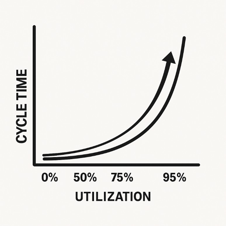
The VUT relationship: utilisation vs. waiting time in plain language

The average waiting time in a station increases by approximately:

(variability) × (u / (1 − u)) × process time

Where as u is the utilisation rate.

Important:

• at 80% occupancy → waiting time ~4× process time (multiplied by a variability factor)

• at 90% occupancy → ~9× processing time

• at 95% occupancy → ~19× processing time

In plain language: every extra percentage point of occupancy above ~85% costs you a disproportionate amount of waiting time.

Typical patterns in practice:

• at 75–80%, the system feels ‘relatively smooth’;

• at 85–90%, every minor disruption becomes noticeable for a long time;

• at 90–95%, you are structurally unable to keep ‘up to date’.

And no: ‘Just plan better’ won’t solve that. You’re working against the laws of physics.

This is why, in work analysis and Lean, the rule of thumb is that you should only schedule/load people up to 80% of their time.

Critical WIP and CONWIP — WIP as the primary controlling variable

Critical WIP (W₀) is the WIP level at which — in an ideal world without variability — you achieve maximum throughput (determined by bottleneck capacity) with minimum lead time (pure processing time).

In the real world, with variability, you want to be just above W₀:

• below W₀ → the bottleneck does not always receive work → throughput drops,

• well above W₀ → extra WIP lengthens lead time without additional output.

CONWIP (Constant Work-In-Process) is a control mechanism that puts this principle into practice:

• you define a maximum WIP at line or system level,

• only when a workpiece leaves the line may a new one enter,

• WIP therefore remains limited and throughput ‘regulates itself’ according to the laws of nature.

Whereas classic Kanban regulates buffers between individual stations, CONWIP regulates the total amount of work in an entire line or factory.

AHA moment: Most factories manage based on throughput (‘more starts = more finished’). Factory Physics teaches you to manage based on WIP. The result is the same throughput level, but with half the chaos.

In summary

• Little’s Law establishes the relationship between WIP, throughput and lead time.

• Variability at or before the bottleneck is the most dangerous.

• The buffering law forces you to make a choice: where do you accept variability?

• High utilisation is not a KPI, but a risk factor.

• WIP caps and CONWIP are practical ways of working within the laws of nature.

If there’s one thing to take away today: don’t look at your average utilisation, but at how often your bottleneck exceeds 90%. That single insight often explains more than ten KPIs put together.

In Article 3, we see how these principles completely reshape daily decisions.